Hilbert 变换
定义
参考 Wikipedia 。
The Hilbert transform of the function $u(t)$ can be thought of as the convolution of $u(t)$ with the function $h(t)=\frac{1}{\pi t}$.
Because $h(t)$ is not integrable, the integrals defining the convolution do not converge. Instead, the Hilbert transform is defined using the Cauchy principal value (denoted here by $p$ ):
$$\mathcal{H}\lbrace u(t)\rbrace=p\int_{-\infty}^{\infty}u(\tau)h(t-\tau)d\tau=\frac{1}{\pi}p\int_{-\infty}^{\infty}\frac{u(\tau)}{t-\tau}d\tau$$
性质
A property of Hilbert transform is: $\mathcal{H}\lbrace\mathcal{H}\lbrace u(t)\rbrace\rbrace=-u(t)$.
解析信号
The analytic signal is constructed from a real signal $f(t)$ and its Hilbert transform $\mathcal{H}\lbrace f(t)\rbrace$ :
$$\tilde f(t)=f(t)-i\mathcal H\lbrace f(t)\rbrace$$
The analytic signal can be written in terms of the instantaneous amplitude $E(t)$ and the instantaneous phase $\phi(t)$ as
$$\tilde f(t)=E(t)e^{i\phi(t)}$$
where
$$\phi(t)=\arctan\frac{\mathfrak I\lbrace\tilde f(t)\rbrace}{\mathfrak R\lbrace\tilde f(t)\rbrace}=\arctan\frac{\mathcal H\lbrace f(t)\rbrace}{f(t)}$$
$$E(t)=\sqrt{\mathfrak R\lbrace\tilde f(t)\rbrace^2+\mathfrak I\lbrace\tilde f(t)\rbrace^2}=\sqrt{f(t)^2+\mathcal H\lbrace f(t)\rbrace^2}$$
共轭转置
定义
即 Hermitian 转置,参考 Wikipedia 。
In mathematics, the conjugate transpose and Hermitian transpose of an $m\times n$ matrix $A$ with complex entries is the $n\times m$ matrix $A^\ast$ obtained from $A$ by taking the transpose and then taking the complex conjugate of each entry.
The definition can also be written as
$$ \left(A^H \right)_{ij} = \overline{A_{ji}} $$
or
$$A^\ast=(\bar{A})^T=\overline{A^T}$$
Another name for the conjugate transpose of a matrix is adjoint matrix.
The commonly used symbols for the conjugate transpose:
- $A^\ast$ or $A^H$ in linear algebra ;
- $A^\dagger$ in quantum mechanics ;
- $A^+$.
例子
If $A=\begin{bmatrix} 1 & -2-i \newline 1+i & i \end{bmatrix} $, then $A^\ast=\begin{bmatrix} 1 & 1-i \newline -2+i & -i \end{bmatrix}$.
Kronecker 乘积
定义
参考 Wikipedia 。
In mathematics, the Kronecker product, denoted by $\otimes$, is an operation on two matrices of arbitrary size resulting in a block matrix. It is a generalization of the outer product from vectors to matrices.
If $A$ is an $m\times n$ matrix and $B$ is a $p\times q$ matrix, then the Kronecker product $A\otimes B$ is the $mp\times nq$ block matrix:
$$A\otimes B=\left[\begin{array}{c} a_{11}B & a_{12}B & \cdots & a_{1n}B \newline a_{21}B & a_{22}B & \cdots & a_{2n}B \newline \vdots & \vdots & \ddots & \vdots \newline a_{m1}B & a_{m2}B & \cdots & a_{mn}B \end{array}\right]$$
where
$$a_{ij}B=\left[ \begin{array}{c} a_{ij}b_{11} & a_{ij}b_{12} & \cdots & a_{ij}b_{1q} \newline a_{ij}b_{21} & a_{ij}b_{22} & \cdots & a_{ij}b_{2q} \newline \vdots & \vdots & \ddots & \vdots \newline a_{ij}b_{p1} & a_{ij}b_{p2} & \cdots & a_{ij}b_{pq} \end{array} \right]$$
例子
$$\left[\begin{array}{c} 1 & 2 \newline 3 & 4 \end{array}\right] \otimes \left[\begin{array}{c} 0 & 5 \newline 6 & 7 \end{array}\right]=\left[\begin{array}{c} 1\cdot \left[\begin{array}{c} 0 & 5 \newline 6 & 7 \end{array}\right] & 2\cdot \left[\begin{array}{c} 0 & 5 \newline 6 & 7 \end{array}\right] \newline 3\cdot \left[\begin{array}{c} 0 & 5 \newline 6 & 7 \end{array}\right] & 4\cdot \left[\begin{array}{c} 0 & 5 \newline 6 & 7 \end{array}\right] \end{array}\right]=\left[\begin{array}{c} 0 & 5 & 0 & 10 \newline 6 & 7 & 12 & 14 \newline 0 & 15 & 0 & 20 \newline 18 & 21 & 24 & 28 \end{array}\right]$$
Frobenius 范数
定义
即 Hilbert-Schmidt 范数,参考 Wikipedia 。
The norm can be defined in various ways:
$$||A||_F=\sqrt{\sum_{i=1}^m\sum_{j=1}^n|a_{ij}|^2}=\sqrt{\text{trace}(A^\dagger A)}=\sqrt{\sum_{i=1}^{\min\lbrace m,n\rbrace}\sigma_i^2(A)}$$
where $A^\dagger$ denotes the conjugate transpose of $A$, and $\sigma_i(A)$ are the singular value of $A$.
Frobenius 内积
参考 Wikipedia 。
$$||A||_F=\sqrt{\langle A,A\rangle_F}$$
where the Frobenius inner product is defined by:
$$\langle A,B\rangle_F=\sum_{i,j}\overline{A_{ij}}B_{ij}=\text{trace}(\overline{A^T}B)$$
Hadamard 乘积
定义
即 Hadamard matrices ,参考 Wikipedia https://en.wikipedia.org/wiki/Hadamard_product_(matrices) 。
For two matrices, $A, B$, of the same dimension, $m\times n$, the Hadamard product, $A\circ B$, is a matrix of the same dimension as the operands, with elements given by
$$(A\circ B)_{i,j}=A_{i,j}B_{i,j}$$
The Hadamard division $A\oslash B$ is defined as:
$$(A\oslash B)_{ij}=\frac{A_{ij}}{B_{ij}}$$
性质
The Hadamard product is commutative, associative and distributive over addition, that is:
- $A\circ B=B\circ A$
- $A\circ(B\circ C)=(A\circ B)\circ C$
- $A\circ(B+C)=A\circ B+A\circ C$
For square matrices $A, B$, the row-sums of their Hadamard product are the diagonal elements of $AB^T$ or $B^TA$:
- $\sum_i(A\circ B)_{i,j}=(B^TA)_{j,j}$
- $\sum_j(A\circ B)_{i,j}=(AB^T)_{i,i}$
Hilbert 矩阵
定义
参考 Wikipedia 。
In linear algebra, a Hilbert matrix is a square matrix with entries being the unit fractions:
$$H_{ij}=\frac{1}{i+j-1}$$
For example, this is the $3\times 3$ Hilbert matrix:
$$H=\left[\begin{array}{c} 1 & \frac{1}{2} & \frac{1}{3} \newline \frac{1}{2} & \frac{1}{3} & \frac{1}{4} \newline \frac{1}{3} & \frac{1}{4} & \frac{1}{5} \end{array}\right]$$
应用
The notoriously ill-conditioned Hilbert matrix can be defined as:
$$J_{ij}:=\begin{cases} \frac{1}{i+j-1} & \text{if }i\text{ mod }j=0\text{, or }j\text{ mod }i=0 \newline 0 & \text{otherwise} \end{cases}$$
For example, if given by $n=5$, the matrix $J$ has the condition number of $4.9\times 10^3$.
矩阵的条件数
矩阵 $A$ 的条件数(condition number)可定义为:
$$\kappa(A)=||A||\cdot ||A^{-1}||$$
如果方阵 $A$ 是奇异的,那么 $A$ 的条件数为正无穷大。实际上,每一个可逆方阵都存在一个条件数。
条件数是一个矩阵(或它所描述的线性系统)的稳定性或敏感度的度量。
A problem with a low condition number is said to be well-conditioned, while a problem with a high condition number is said to be ill-conditioned.
积分函数表
参考 Wikipedia。
另外,这里还有在线数学笔记。
Dirac comb 函数
即 Shah 函数,参考 Wikipedia 。
在数学上,Dirac comb 即一个由 Dirac delta 函数构成的周期性调和分布(periodic tempered distribution)。也即电子工程中的脉冲序列(impulse train)或采样函数(sampling function)。
A Dirac comb is an infinite series of Dirac delta functions spaced at intervals of $T$.
函数表达式为:
$$III_T(t)=\sum_{k=-\infty}^\infty \delta (t-kT)$$
函数图像如下:

Euclidean 距离 vs Manhattan 距离
Euclidean 距离
即欧几里德长度、毕达哥拉斯度量(Pythagorean metric)或 $L^2$ 距离,参考 Wikipedia 。
In mathemactics, the Euclidean distance is the “ordinary” straight-line distance between two points in Euclidean space.
In Cartesian coordinates, if $\textbf p = (p_1, p_2, \ldots, p_n)$ and $\textbf q = (q_1, q_2, \ldots, q_n)$ are two points in Euclidean n-space, then the Euclidean distance from $\textbf p$ to $\textbf q$, or from $\textbf q$ to $\textbf p$ is given by the Pythagorean formula:
$$ d (\textbf p, \textbf q) = d (\textbf q, \textbf p) = \sqrt{ \sum_{i = 1}^n (q_i - p_i)^2 } $$
Manhattan 距离
即曼哈顿长度、出租车距离(taxicab metric / taxicab distance)、rectilinear distance、snake distance、city block distance 或 $L^1$ 距离,参考 Wikipedia 。
A taxicab geometry is form of geometry in which the distance between two points is the sum of the absolute differences of their Cartesian coordinates.
The taxicab distance between two points, $\textbf p = (p_1, p_2, \ldots, p_n)$ and $\textbf q = (q_1, q_2, \ldots, q_n)$, in an n-dimensional space with fixed Cartesian coordinate system, is the sum of the lengths of the projections of the line segment between the points onto the coordinate axes:
$$ d (\textbf p, \textbf q) = \lVert \textbf p - \textbf q \rVert_1 = \sum_{i = 1}^n \lvert p_i - q_i \rvert $$
二者差异
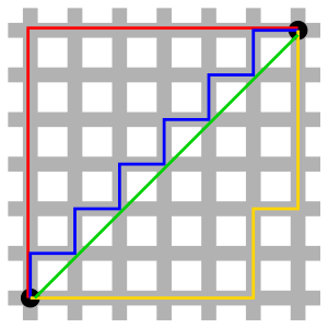
In taxicab geometry, the red, yellow, and blue paths all have the same shortest path length of 12. In Euclidean geometry, the green line has length $ 6\sqrt{2} \approx 8.49 $ and is the unique shortest path.
Monte Carlo 积分
参考 Wikipedia 。
概述
In mathematics, Monte Carlo integration is a technique of numerical integration using random numbers. It is a particular Monte Carlo method that numerically computes a definite integral. This method is particularly useful for higher-dimensional integrals.
Monte Carlo integration employs a non-deterministic approach: each realization provides a different outcome. In Monte Carlo, the final outcome is an approximation of the correct value with respective error bars, and the correct value is likely to be within those error bars.
公式化表达
The problem Monte Carlo integration addresses is the computation of a multidimensional definite integral
$$ I = \int_\Omega f(\mathbf x) d\mathbf x $$
where $\Omega$, a subset of $\mathbf R^m$, has volume
$$ V = \int_\Omega d\mathbf x $$
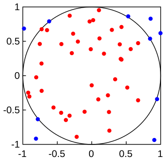
The naive Monte Carlo approach is to sample points uniformly on $\Omega$: given $N$ uniform samples $\mathbf x_1, \mathbf x_2, \ldots, \mathbf x_N \in \Omega$, $I$ can be approximated by
$$ I \approx Q_N \equiv V \frac{1}{N} \sum_{i = 1}^N f(\mathbf x_i) = V \langle f \rangle $$
This is because the law of large numbers ensures that $\lim_{N \rightarrow \infty} Q_N = I$.
Heaviside 阶跃函数
即单位阶跃函数,参考 Wikipedia。
概述
The Heaviside step function, usually denoted by $H$ (but sometimes $u$), is a discontinuous function, whose value is zero for negative arguments and one for positive arguments.
The Heaviside function can also be defined as the integral of the Dirac delta function:
$$ H(x) = \int_{ - \infty}^x \delta(s) ds $$
离散形式
An alternative form of the unit step, as a function of a discrete variable $n$:
$$ H[n] = \begin{cases} 0, & n < 0 \newline 1, & n \geq 0 \end{cases} $$
or using the half-maximum convention:
$$ H[n] = \begin{cases} 0, & n < 0 \newline \frac{1}{2}, & n = 0 \newline 1, & n > 0 \end{cases} $$
where $n$ is an integer.
The discrete-time unit impulse is the first difference of the discrete-time step
$$ \delta[n] = H[n] - H[n - 1] $$
多目标最优化
即矢量最优化、Pareto 最优化、multicriteria 最优化或 multiattribute 最优化,参考 Wikipedia。
概述
Multi-objectvie optimization is an area that is concerned with mathematical optimization problems involving more than one objective function to be optimized simultaneously, where optimal decisions need to be taken in the presence of trade-offs between two or more conflicting objectives.
Pareto 解
For a nontrivial multi-objective optimization problem, no single solution exists that simultaneously optimizes each objective. In that case, the objective functions are said to be conflicting, and there exists a (possibly infinite) number of Pareto optimal solutions.
A solution is called nondominated or Pareto optimal solution, if none of the objective functions can be improved in value without degrading some of the other objective values. Without additional subjective preference information, all Pareto optimal solutions are considered equally good.
Pareto 前沿

In mathematical terms, a feasible solution $x_1 \in X$ is said to (Pareto) dominate another solution $x_2 \in X$, if
$$ \begin{cases} f_i(x_1) \leq f_i(x_2) & \text{ for all indices } i \in {1, 2, \ldots, k} \newline f_j(x_1) < f_j(x_2) & \text{ for at least one index } j \in {1, 2, \ldots, k} \end{cases} $$
where $k \geq 2$ is the number of objectives.
A solution $x_\ast \in X$ (and the corresponding outcome $f(x_\ast)$) is called Pareto optimal, if there does not exist another solution that dominates it. The set of Pareto optimal outcomes is called the Pareto front or Pareto boundary.
Helmholtz 方程
定义
参考 Wikipedia。
In mathematics, the eigenvalue problem for the Laplace operator is known as the Helmholtz equation. It corresponds to the linear partial differential equation:
$$ \nabla^2 f = - k^2 f $$
where $\nabla^2$ is the Laplace operator, $k^2$ is the eigenvalue, and $f$ is the eigenfunction.
When the equation is applied to waves, $k$ is knows as the wave number.
波动方程
对于声速恒为 $c$ 的均匀介质,由源 $f(\mathbf x_0, t)$ 激发的压力场 $p(\mathbf x, t)$ 满足声波波动方程
$$ \nabla^2 p(\mathbf x, t) - \frac{1}{c^2} \frac{\partial^2 p(\mathbf x, t)}{\partial t^2} = f(\mathbf x_0, t) $$
转化到频率域即
$$ \nabla^2 P(\mathbf x, \omega) + \frac{\omega^2}{c^2} P(\mathbf x, \omega) = F(\mathbf x_0, \omega) $$
也即
$$ \nabla^2 P + k^2 P = F $$
其中 $k = \omega / c$ 为波数。
Green 函数
参考 Wikipedia。
非均匀 Helmholtz 方程(Inhomogeneous Helmholtz equation)的 Green 函数满足:
$$ \nabla^2 G(x) + k^2 G(x) = - \delta(x) \in \mathbb{R}^n $$
其解为:
$$ G(x) = \begin{cases}
\frac{i e^{i k |x|}}{2 k}, & n = 1 \newline
\frac{i}{4} H_0^{(1)}(k |x|), & n = 2 \newline
\frac{e^{i k |x|}}{4 \pi |x|}, & n = 3 \newline
\end{cases} $$
其中 $H_0^{(1)}$ 为第一类零阶 Hankel 函数。
特殊矩阵
Toeplitz 矩阵
参考 Wikipedia。
In linear algebra, a Toeplitz matrix or diagonal-constant matrix is a matrix in which each descending diagonal from left to right is constant.
A Toeplitz matrix $ \mathbf A $ by $ n \times n $ is of the form
$$ \mathbf A = \begin{bmatrix}
a_0 & a_{ - 1} & a_{ - 2} & \cdots & \cdots & a_{ - (n - 1)} \newline
a_1 & a_0 & a_{ - 1} & \ddots & \ddots & \vdots \newline
a_2 & a_1 & \ddots & \ddots & \ddots & \vdots \newline
\vdots & \ddots & \ddots & \ddots & a_{ - 1} & a_{ - 2} \newline
\vdots & \ddots & \ddots & a_1 & a_0 & a_{ - 1} \newline
a_{n - 1} & \cdots & \cdots & a_2 & a_1 & a_0 \newline
\end{bmatrix} $$
If the $ i, j $ element of $ \mathbf A $ is denoted $ A_{i, j} $, then $ A_{i, j} = A_{i + 1, j + 1} = a_{i - j}$.
A Toeplitz matrix is not necessarily square.
Hankel 矩阵
参考 Wikipedia。
In linear algebra, a Hankel matrix or catalecticant matrix is a square matrix in which each ascending skew-diagonal from left to right is constant.
A Hankel matrix $ \mathbf A $ by $ n \times n $ is of the form
$$ \mathbf A = \begin{bmatrix}
a_0 & a_1 & a_2 & \cdots & \cdots & a_{n - 1} \newline
a_1 & a_2 & a_3 & \ddots & \ddots & \vdots \newline
a_2 & a_3 & \ddots & \ddots & \ddots & \vdots \newline
\vdots & \ddots & \ddots & \ddots & a_{2n - 5} & a_{2n - 4} \newline
\vdots & \ddots & \ddots & a_{2n - 5} & a_{2n - 4} & a_{2n - 3} \newline
a_{n - 1} & \cdots & \cdots & a_{2n - 4} & a_{2n - 3} & a_{2n - 2} \newline
\end{bmatrix} $$
If the $ i, j $ element of $ \mathbf A $ is denoted with $ A_{i, j} $, and assuming $ i \le j $, then $ A_{i, j} = A_{i + k, j - k} $ for all $ k = 0, 1, \ldots, j - i $.
循环矩阵
即 circulant matrix,参考 Wikipedia。
In linear algebra, a circulant matrix is a square matrix in which each row vector is rotated one element to the right relative to the preceding row vector.
A circulant matrix $ \mathbf A $ by $ n \times n $ is of the form
$$ \mathbf A = \begin{bmatrix}
a_0 & a_{n - 1} & a_{n - 2} & \cdots & a_2 & a_1 \newline
a_1 & a_0 & a_{n - 1} & \ddots & \ddots & a_2 \newline
a_2 & a_1 & \ddots & \ddots & \ddots & \vdots \newline
\vdots & \ddots & \ddots & \ddots & a_{n - 1} & a_{n - 2} \newline
a_{n - 2} & \ddots & \ddots & a_1 & a_0 & a_{n - 1} \newline
a_{n - 1} & a_{n - 2} & \cdots & a_2 & a_1 & a_0 \newline
\end{bmatrix} $$
Vandermonde 矩阵
参考 Wikipedia。
In linear algebra, a Vandermonde matrix is a matrix with the terms of a geometirc progression in each row.
A Vandermode matrix $ \mathbf A $ by $ m \times n $ is of the form
$$ \mathbf A = \begin{bmatrix}
1 & a_1 & a_1^2 & \cdots & a_1^{n - 1} \newline
1 & a_2 & a_2^2 & \cdots & a_2^{n - 1} \newline
\vdots & \vdots & \vdots & \ddots & \vdots \newline
1 & a_m & a_m^2 & \cdots & a_m^{n - 1} \newline
\end{bmatrix} $$
If the $ i, j $ element of $ \mathbf A $ is denoted with $ A_{i, j} $, then $ A_{i, j} = a_i^{j - 1} $.
Cauchy 矩阵
参考 Wikipedia。
In mathematics, a Cauchy matirx is an $ m \times n $ matrix with element $ a_{ij} $ in the form
$$ a_{ij} = \frac{1}{x_i - y_j}; x_i - y_j \ne 0, 1 \le i \le m, 1 \le j \le n $$
where $ x_i $ and $ y_j $ are elements of a field $ \mathcal F $.
Every submatrix of a Cauchy matrix is itself a Cauchy matrix.
交换矩阵
即 exchange matrix,参考 Wikipedia。
In mathematics, especially linear algebra, an exchange matrix (also called the reversal matrix, backward identity, or standard involutory permutation) is a matrix where the 1 element resides on the counterdiagonal and all other elements are zero.
An exchange matrix $ \mathbf A $ by $ n \times n $ is of the form
$$ \mathbf A = \begin{bmatrix}
0 & 0 & \cdots & 0 & 0 & 1 \newline
0 & \ddots & \ddots & 0 & 1 & 0 \newline
\ldots & \ddots & \ddots & \ddots & 0 & 0 \newline
0 & 0 & \ddots & \ddots & \ddots & \ldots \newline
0 & 1 & 0 & \ddots & \ddots & 0 \newline
1 & 0 & 0 & \cdots & 0 & 0 \newline
\end{bmatrix} $$
If the $ i, j $ element of $ \mathbf A $ is denoted with $ A_{i, j} $, then
$$ A_{i, j} = \begin{cases}
1, & j = n - i + 1 \newline
0, & j \ne n - i + 1 \newline
\end{cases} $$
Wolfe 条件
参考 Wikipedia。
概述
In the unconstrained minization problem, the Wolfe conditions are a set of inequalities for performing inexact line search, especially in quasi-Newton methods.
The inexcat line searches provide an efficient way of computing an acceptable step length that reduces the objective function ‘sufficiently’, rather that minimizing the objective function over the whole positive real space exactly.
Armijo 规则和曲率条件
A step length $ \alpha_k $ is said to satisfy the Wolfe conditions, restricted to the direction $ \mathbf{p}_k $, if the following two inequalities hold:
$$ \begin{cases} f (\mathbf{x}_k + \alpha_k \mathbf{p}_k) \leqslant f(\mathbf{x}_k) + c_1 \alpha_k \mathbf{p}_k^{\mathrm T} \nabla f(\mathbf{x}_k), & \text{known as the Armijo rule} \newline \mathbf{p}_k^{\mathrm T} \nabla f(\mathbf{x}_k + \alpha_k \mathbf{p}_k) \leqslant - c_2 \mathbf{p}_k^{\mathrm T} \nabla f(\mathbf{x}_k), & \text{known as the curvature condition} \end{cases} $$
with $ 0 < c_1 < c_2 < 1 $, where $ c_1 $ is usually chosen to be quite small and $ c_2 $ is much larger. Nocedal and Wright (1999, Numerical Optimization) give example value of $ c_1 = 10^{ - 4} $ and $ c_2 = 0.9 $ for Newton or quasi-Newton methods, and $ c_2 = 0.1 $ for the nonlinear conjugate gradient method.
The Armijo rule ensures that the step length decreases the objective function ‘sufficiently’, and the curvature condition ensures that the slope has been reduced sufficiently. The two conditions can be interpreted as respectively providing an upper and lower bound on the acceptable step length values.
强 Wolfe 条件
If we modify the curvature condition to the following:
$$ | \mathbf{p}_k^{\mathrm T} \nabla f(\mathbf{x}_k + \alpha_k \mathbf{p}_k) | \leqslant c_2 | \mathbf{p}_k^{\mathrm T} \nabla f(\mathbf{x}_k) | $$
then the Armijo rule and the above inequality form the so-called strong Wolfe conditions, and force $ \alpha_k $ to lie close to a critical point (i.e., a point in the domain of the function where the function is either not differentiable or the derivative is equal to zero) of the function $ \varphi(\alpha) = f(\mathbf{x}_k + \alpha \mathbf{p}_k) $.